Spreadsheets
The VisiCalc spreadsheet
program, introduced in 1979 to run on the Apple II computer, was considered to
be the single most important reason why microcomputers gained acceptance in the
business world. Lotus 1-2-3, developed by
Mitch Kapor, was introduced
in 1983 and quickly became the number one selling spreadsheet software on the
IBM compatible PC platform. Within a few short years, Lotus 1-2-3 had sold over
a million copies of its software package. Many people purchased computers just
so that they could run Lotus 1-2-3.
Lotus was to spreadsheets what Word
Perfect was to word processing - both, the number one program in its
category, and thus the standard. Just as word processing files are called
documents, spreadsheet files are called worksheets. Today, the entire file in
Excel is called a workbook, while each sheet is called a worksheet. Other
spreadsheet programs include Quattro Pro, and Works Spreadsheet.
Spreadsheets contain a grid of rows and columns. Rows (the horizontal part of
a worksheet) are numbered from 1 to 65,536 (in Excel 2000) and from 1 to 16,384
(in Works 4.5). Older versions of Lotus 1-2-3 were numbered from 1 to 8192.
Actually, the earlier DOS version of Lotus went from 1 to 2048. Columns (the
vertical part of a worksheet) are lettered from A to IV. After the column
letters go from A, B, C, ... to Z, they use two letters, AA, AB, AC, ... to AZ,
then use BA, BB, BC, BD... to BZ, and stop on the 256th column which is lettered
IV.
Cell - The intersection of a row and a column. Each cell has a unique
location name called a cell address.
Cell Address - is made up of the column letter, plus the row number.
For example, the top left cell in a worksheet has the cell address A1. The top
right corner of the worksheet has the cell address IV1. The bottom left corner
of the worksheet has the cell address A65536 and the bottom right is IV16636.
Active Cell - the cell which has focus. The cell with the bold border
around it - called the cell pointer. When we type, the information is placed
into the active cell.
Cell Pointer Movement Keys: Arrow Up, Arrow Down, Arrow Left, and
Arrow Right move the cell pointer one cell Up, Down, Left and Right. The HOME
key moves the cell pointer to column A in the current row. In Excel, the TAB key
moves the cell pointer one cell to the right, while SHIFT + TAB moves the cell
pointer one cell to the left. Lotus uses TAB key to move one screen to the right
and the SHIFT + TAB keys to move one screen to the left. Page Up moves the cell
pointer one screen up, while Page Down moves the cell pointer one screen down.
After pressing the END key, you can tap any of the four arrow keys to move to
the end of contiguous cells in the direction of the arrow. Note that the END key
is a toggle key - it toggles on and off the END feature, indicated by the word
END on the status bar.
Modes: It is important to be aware of the mode you are in when you are
working with a spreadsheet program. This is because several keys act differently
depending upon the mode you are in. The cell pointer movement keys listed above,
assume you are in READY mode.
Before you can type information into a cell in Excel, you must be in READY
mode. The mode indicator is in the lower left corner of the screen on the status
bar. After you begin typing information into a cell in Excel, you change to
ENTER mode. After you type information, you can press the ENTER key or press
one of the four arrow keys to place your information into the active cell -
which also returns you to ready mode.
Often you will edit the contents of a cell by pressing the F2 (Edit key) or
by clicking on the cell contents line (or formula bar) at the top of the screen.
When you begin changing information in a cell, the spreadsheet program switches
you to EDIT mode. Note the word EDIT in the status bar.
Once in EDIT mode, your left and right arrow keys act differently. The left
and right arrow keys act on the edit line, just like they do in a word
processing program - allowing you to move a character to the left or a character
to the right. The Backspace and Delete key also act differently in EDIT mode -
They erase a character to the left or right, just like they do in a word
processor. In READY mode, the Backspace key erases the contents of the cell and
puts you in EDIT mode. The Delete key in READY mode erases the contents of the
cell and returns you to READY mode.
When editing a cell in Excel, you can tap the ESC (escape) key
to cancel your changes and return to READY mode.
Earlier versions of Lotus 1-2-3 used a menu system which started by the user
pressing the slash key ( / ). For example, the user would save a file, accessing
the menu mode, by pressing /FSY. These keystrokes would enter menu mode ( / ),
then select File (F), the select save (S), and finally select Yes I want to save
(Y). Versions of Excel, prior to Excel 97, used the slash key ( / ) for Excel
help for Lotus users. Sometimes users would accidentally press the slash key ( /
) and continue to type other letters which happened to match Lotus menu item
letters. To exit this menu system, and return to ready mode, the user can press
the ESC (escape) key several times. Excel 2000 uses the slash key ( / ) to
change focus to the menu bar (same as the ALT key) so it is quite possible that
you may want to exit commands deep into the Excel 2000 menu system by using the
ESC (escape) key.
POINT mode allows the user to point to cell references, rather than
having to type in the cell address. To enter point mode, start a formula or
function just as you normally would - and when you get ready to type a cell
address, instead, use the arrow keys or Page Up/Page Down keys or HOME key, etc.
to move to the cell you're about to reference in your formula or function. Once
you point to the cell, press the next operator, parenthesis, comma or just press
the ENTER key if you are finished with the formula. Using point mode to enter
cell addresses will speed up the process of creating a spreadsheet since it will
increase your accuracy. It should eliminate common errors caused by entering the
wrong cell address.
Recalculation of the Worksheet: Unless you have changed the default
recalculation setting, Excel recalculates your entire worksheet each time you
change the contents of a cell. This means that all cells that are calculated
based on the value of a changed cell, will also change.
Value vs. Label: You can enter values or labels into a cell. A value
is a number which has numerical value - one that can be calculated such as
added, subtracted, multiplied, or divided. Values can be a number, a formula, or
a function. Labels are any words such as headings, descriptions, addresses,
notes, etc. Labels cannot be added, subtracted, multiplied or divided. Excel
automatically treats entries as labels if you type a letter to begin the entry
in the cell. If you begin an entry in a cell with a number, then type a space or
other letter after the number, Excel treats your entry as a label.
If you type a formula into a cell (such as A1+B1), Excel treats your entry as
a label since you started your entry with the letter A. This is not what you
wanted. To force Excel to treat your formula as a value, you must start the
entry with the equal sign (=) or a plus sign (+). Instead, in order to get Excel
to treat your formula as a value, you would enter this formula as =A1+B1 or
+A1+B1.
Formula - a user created calculation to define cells in relation to
other cells in a worksheet. Formulas calculate values in a specific order. A
formula in Microsoft Excel always begins with an equal sign (=). The equal sign
tells Excel that the succeeding characters constitute a formula. You can also
start a formula with the plus sign (+), as you do in Lotus 1-2-3. Excel will
automatically add the equal sign (=) in front of your formula. Following the
equal sign are the elements to be calculated (the operands), which are separated
by calculation operators. Excel calculates the formula from left to right,
according to a specific order for each operator in the formula. You can change
the order of operations by using parentheses.
Order of Operations and Operators: Excel is programmed to follow the
same math rules we learned to follow when it encounters a formula with several
operations. For this reason, we must understand the math rule so that we'll know
how Excel will calculate a formula.
| Easy to Remember |
Operation |
Operator |
| Please |
Parentheses |
( ) parenthesis |
| Excuse |
Exponents |
^ caret |
| My Dear |
Multiplication and Division |
* multiplication
/ division (forward /) |
| Aunt Sally |
Addition and Subtraction |
+ addition
- subtraction |
Example #1: If we typed +100*.05+4/2 into a cell, what value would be
displayed - would it be 7 or 4.5?
Example #2: If we typed +200+50/5*4-20 into a cell, what value would be
displayed - would it be 180 or 220?
(answers at the bottom of this page)
Keep in mind that the arithmetic operators for addition, subtraction,
multiplication and division are located on the numeric keypad on the right side
of the keyboard. Knowing this could help you on an exam if you were trying to
remember if the arithmetic operator for division was a back slash or a forward
slash. Also, note that the caret (^ - is a shift and the number 6 key) is used
to raise a number to a power. To enter 53 we would simply type +5^3
in a cell.
Range - a group of cells in the shape of a rectangle, identified by
two opposite corners. In Excel we define a range by including the cell addresses
of two opposite corners with a colon in between. For example, to describe the
range of cells including A1, A2, A3, B1, B2, and B3, we would use A1:B3. We
could also describe the same range with B3:A1, or B1:A3, or A3:B1. Other
spreadsheet programs are similar. Lotus 1-2-3 uses two periods between cell
addresses in the same way; A1..B3, etc.
Functions - built in computations such as mathematical, financial,
statistical, logical, etc. Excel 2000 has over 200 built in functions. Functions
are predefined formulas that perform calculations by using specific values,
called arguments, in a particular order, or structure.
Arguments - values that you give functions.
For example, the SUM function adds values or ranges of cells, and the PMT
function calculates the loan payments based on an interest rate, the length of
the loan, and the principal amount of the loan.
The SUM, MAX, MIN, AVERAGE functions are similar in that they require only
one argument - the range. The syntax is =SUM(range). We enter the function
exactly as =SUM(A1:B3) to add to total of all values in the range A1:B3. The MAX
function displays the highest number in the range. The MIN function displays the
lowest value in the range. And, the AVERAGE function returns the average of the
numbers in the specified range.
The syntax of the payment function is =PMT(interest, term, principal). This
function has three arguments. Arguments are separated by commas and must be in
the exact order required by the function. Also, we must enter all arguments in
the same form - ie: if we are computing a monthly payment, we must enter the
interest rate as a monthly interest rate and we must enter the term of the loan
in months.
The syntax of the IF function is =IF(condition, true, false). Enter the
condition you want to test as the first argument. Then, enter the value (or
formula) you want displayed if the condition is true, and another for the false
condition. This is a great formula for payroll applications. It is often used to
test for overtime - testing for hours over 40. You can use nested IF statements
(IF statements inside other IF statements) to calculate federal income taxes
based on the withholding allowances and income tax brackets.
Once you learn to use these few functions, you will know how to use the rest
of the more than 200 built in functions. In order to use any of the other
functions, take a quick look at the help feature to learn the exact syntax. They
all work the same way.
As in other Windows applications, the F1 key is the help key.
Three Mouse Pointers in Excel:
- Fat Cross - used to select a cell or a range of cells. To get the
mouse pointer to change into the Fat Cross, position the mouse pointer
anywhere in the active cell that is not on the bottom right corner or on the
exact edge of the active cell.
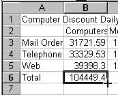
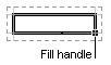
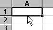
- Thin Cross - used to copy or fill a range of cells. To get the
mouse pointer to change into the Thin Cross, position the mouse pointer on
the bottom right edge of the active cell or a selected range.
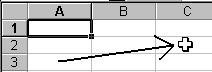
- Arrow - used to move a cell or a range of cells.
Since the introduction of Office XP, Excel 2002 now displays a Four
Headed Arrow to move a cell or range of cells.

To get the mouse pointer to change into the Arrow, position the mouse
pointer on the exact edge of the active cell or selected range - but not in
the bottom right corner.
Answer to Example #1 is 7 since we must perform
multiplication and division, before we add and subtract. Must divide 4/2 before
we add it to the product of 100*.05 to get 5 + 2 = 7 as our answer.
Answer to Example #2 is 220 since we must first take 50/5 and get 10,
then multiply it by 4 to get 40. All this must be calculated BEFORE we add it
all together with 200 + 40 - 20 to get 220 as the answer.